Expected Values, Bernoulli, and Binomial Variables
Expected Values of Discrete Random Variables
The expected value of a discrete random variable X is equal to the sum of each value of the random variable multiplied by its probability.
μ = E(X) = ∑xxP(x)
| x |
P(x) |
xP(x) |
| 0 |
0.2 |
0 |
| 1 |
0.1 |
0.1 |
| 2 |
0.2 |
0.4 |
| 3 |
0.1 |
0.3 |
| 4 |
0.3 |
1.2 |
| 5 |
0.1 |
0.5 |
|
2.5 = E(X) = μ |
Variance and Standard Deviation of a Random Variable
The variance of a random variable is defined as the expected squared deviation from the mean:
σ2 = V(X) = E[(X-μ)2] = ∑x(x-μ)2P(x)
As usual, the standard deviation of a random variable is the square root of its variance: σ = SD(X)
Example: Let's the previous example where μ = 2.5
| x |
P(x) |
xP(x) |
(x− μ) |
(x− μ)2 |
(x− μ)2P(x) |
| 0 |
0.2 |
0 |
− 2.5 |
6.25 |
1.25 |
| 1 |
0.1 |
0.1 |
− 1.5 |
2.25 |
0.225 |
| 2 |
0.2 |
0.4 |
− 0.5 |
0.25 |
0.05 |
| 3 |
0.1 |
0.3 |
0.5 |
0.25 |
0.025 |
| 4 |
0.3 |
1.2 |
1.5 |
2.25 |
0.675 |
| 5 |
0.1 |
0.5 |
2.5 |
6.25 |
0.625 |
|
2.5 = E(X) = μ |
|
|
|
2.8 |
So, the standard deviation σ = 1.688
Bernoulli Random Variable
If an experiment consists of a single trial and the outcome can only be: Success or Failure. In this case the
trial is called a Bernoulli trial.
The number of success X in one Bernoulli trial, which can be 1 or 0, is called a Bernoulli random variable.
Let's assume p is the probability of success in a Bernoulli experiment, the E(X) = p and V(X) = p(1 − p).
The Binomial Random Variable
Assuming a Bernoulli Process including a sequence of n identical trials satisfying the following conditions:
- Each trial has two possible outcomes: Success and Failure, which are mutually exclusive and exhaustive.
- The probability of success, p, does not change from trial to trial.
The probability of failure, q, is equal to 1 − p.
- All of the n trials in the Bernoulli process are independent, where
the outcome of any trial does not have any impact on other trials.
A random variable, X, representing the number of successes in n Bernoulli trials,
and the probability p of success in any given trial is said to follow the binomial probability distribution
with parameters n and pp. X here is called the binomial random variable.
The binomial formula is as follows:
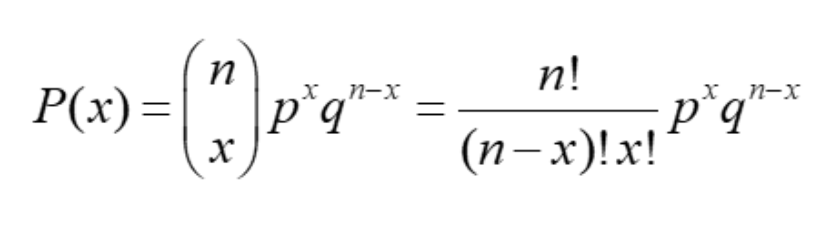
where:
- n: the number of trials
- x: the number of successes or the number being sampled
- p: the probability of success in a one trial
- q = 1 − p, the probability of failure in a one trial
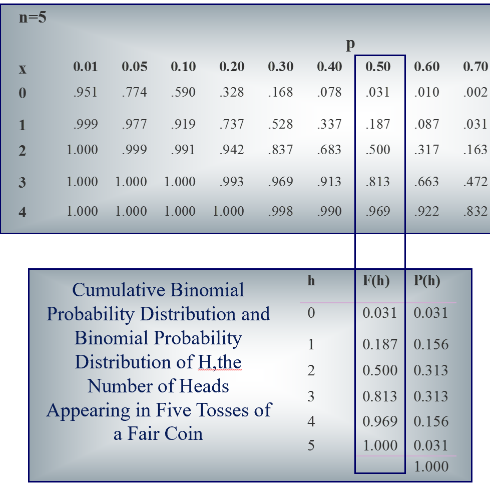
Deriving Individual Probabilities from Cumulative Probabilities
F(X) and P(X) are the cumulative binomial probability distribution and
the binomial probability distribution of X respectively.
F(X) = P(X ≤ x) = ∑i ≤ x P(i)
P(X) = F(x) − F(x − 1);
Example: Calculate P(3).
Answer: P(3) = F(3) − F(2) = 0.813 − 0.50 = 0.313 (based on table lookup see below)
Mean, Variance, and Standard Deviation of the Binomial Distribution
Mean of a binomial distribution: E(X) = μ = np
Variance of a binomial distribution: σ2 = V(X) = npq
Standard deviation of a binomial distribution: σ = SD(X) =
√ npq
Example:
Assume T counts the number of tails in five tosses of a fair coin:
σT = E(T) = 5 × 0.5 = 2.5
σT2 = V(T) = 5 × 0.5 × 0.5 = 1.25
σT = SD(T) =
√ 1.25
= 1.118
Continuous Random Variables
A continuous random variable is a random variable that can take on any value in an interval of numbers.
The probabilities associated with a continuous random variable X are determined by the probability density function of
the random variable. The function f(x) has the following properties:
- f(x) ≥ 0 for all x
- The probability that X will be between two numbers a and b is equal to the area under f(x) between a and b
- The total area under the curve of f(x) is equal to 1.00
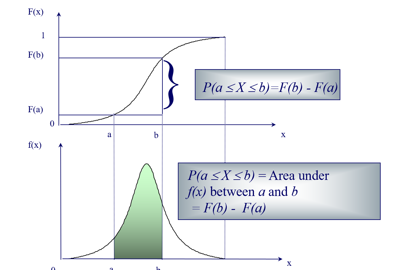
F(x) denotes the cumulative distribution function of a continuous random variable.
F(x) = P(X ≤ x) = Area under f(x) between the smallest possible value of X (often ∞) and the point x.
The illustration of probability density function and cumulative distribution function is shown below:
For more details, please contact me here.