Introduction to Change in Selling Price
Introduction
Here we will look at the effects of changes in selling price, fixed costs, and variable costs on the net income and break-even point.
The use of graphs can also help us with break-even analysis.
We usually call the graph showing the total revenue and the total cost graphs together a break-even chart.
This chart is an easy visual way to analyze the financial position of a business for different number for units
sold (sales volume) or produced (volume of output).
We can see at a glance the amount of profit or loss that is generated for different levels of sales or production.
Change in Selling Price
A change in the selling price per unit will cause a change in the total revenue equation.
An increase in the selling price will cause an increase in the total revenue;
the TR graph will have a greater slope. A decrease in the selling price will cause a decrease in the total revenue;
the TR graph will have a smaller slope.
The higher the selling price, the lower the level of the break-even point and
the higher the profit level provided that the variable costs and the fixed costs remain the same.
Example:
The graph shows the effect of an increase and a decrease in the selling price per unit.
TC is the total cost graph.
The graph below shows this effect:
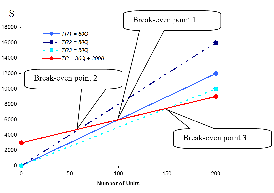
The graphs depicts the following:
- The TR1 graph has a slope of 60. Its equation is TR1 = 60Q. The selling price per unit is $60.
- The TR2 graph has a slope of 80. Its equation is TR2 = 80Q. The selling price per unit is $80.
- The TR3 graph has a slope of 50. Its equation is TR3 = 50Q. The selling price per unit is $50.
- The break-even point is lower for TR2 and higher for TR3.
Example 2:
Please access the following link to do a similar exercise about change in selling price:
Change Selling Price exercise with solution
Learning Further details on Change in Variable Costs is available through the link.
For more details, please contact me here.